Metal fatigue failures happen without warning, often at stress levels well below what engineers expect. Your carefully calculated safety margins become meaningless when microscopic cracks grow silently through critical components, leading to catastrophic failures that could have been prevented.
Metal fatigue analysis requires a systematic 20-step approach that covers stress-life curves, strain-life methods, fracture mechanics, environmental factors, and practical design strategies to predict and prevent fatigue failures in engineering components.

This guide walks you through each essential step, from understanding why metals fail below yield strength to implementing real-world solutions. You’ll learn proven methods that help you design components that last, backed by practical examples from aerospace and automotive industries.
Why does metal fatigue occur below yield strength?
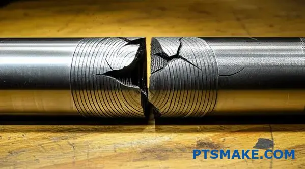
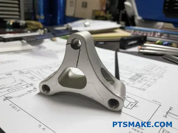
Have you ever seen a metal part snap unexpectedly? It might have seemed strong, handling its load just fine. The culprit is often metal fatigue.
This isn’t about a single, overwhelming force. It’s the silent accumulation of damage. Repeated stress cycles, even small ones, are the cause. They create microscopic flaws that grow over time.
The Two Failure Paths
This process is fundamentally different from a static overload failure. The distinction is crucial for designing durable parts.
| Feature | Static Failure | Fatigue Failure |
|---|---|---|
| Load Type | Single, high load | Repeated, cyclic load |
| Stress Level | Above yield strength | Often below yield strength |
| Onset | Sudden | Gradual, cumulative |
A Look at the Microscopic Level
The answer lies deep within the metal’s crystal structure. On a large scale, the stress is in the elastic range. This means the part should return to its original shape.
But at the microscopic level, a different story unfolds. The metal’s crystal lattice contains imperfections called dislocations. Cyclic loading causes these dislocations to move and cluster together.
The Birth of a Crack
This concentrated movement creates tiny areas of localized plastic deformation. These zones are known as persistent slip bands1. They form tiny steps, like extrusions and intrusions, on the material’s surface.
These surface imperfections act as stress concentrators. They become the starting points for microscopic cracks. With each stress cycle, the crack grows a little bit more. At PTSMAKE, understanding this mechanism is key to our material selection process. It ensures the parts we machine can withstand their intended service life.
| Scale | Observation | Implication |
|---|---|---|
| Macroscopic | Part appears elastic, no visible change. | Engineers might assume it’s safe. |
| Microscopic | Localized plastic deformation occurs. | Damage accumulates, initiating cracks. |
In short, metal fatigue is a cumulative process. Repeated stresses, even those below the yield point, cause localized microscopic damage. This damage grows into cracks that lead to eventual failure, distinguishing it from sudden static overload.
What is a Stress-Life (S-N) curve?
An S-N curve, or Stress-Life curve, is a fundamental tool in engineering. It graphically represents a material’s fatigue life.
The curve plots the magnitude of a cyclic stress (S) against the number of cycles to failure (N).
Understanding the Axes
The vertical axis shows the stress level. The horizontal axis, often on a logarithmic scale, shows the number of cycles. This helps us visualize how a part wears out over time. It’s crucial for predicting and preventing metal fatigue.
A simple way to look at it is:
| Stress Level | Cycles to Failure |
|---|---|
| High Stress | Fewer Cycles |
| Low Stress | Many Cycles |
This relationship helps us design parts that will last for their intended service life without failing unexpectedly.
The Endurance Limit: Designing for Infinite Life
The most critical feature of an S-N curve for certain materials is the endurance limit. This concept is a game-changer for long-term reliability.
The endurance limit is the stress level below which a material can withstand a very large, almost infinite, number of load cycles without failing. The curve essentially becomes horizontal at this point.
However, not all materials have this property.
| Material Group | Common Endurance Limit Behavior |
|---|---|
| Steel and Titanium Alloys | Often exhibit a distinct endurance limit. |
| Aluminum and Copper Alloys | Typically do not have a clear limit. |
For materials like steel, if we design a component so that its operating stresses are always below the endurance limit, it can theoretically last forever. This is the foundation of ‘infinite life’ design. In past projects at PTSMAKE, understanding this distinction is key. For a steel part on industrial machinery, we aim for infinite life. The fatigue strength coefficient2 helps us model this behavior accurately. For an aluminum aircraft part, the design must account for a finite lifespan and regular inspections.
The S-N curve maps stress to a material’s cycle life. Its most important feature for many metals is the endurance limit. This limit is the key to designing components that can withstand cyclic loading indefinitely, preventing long-term metal fatigue.
What is the role of stress concentrations?
In engineering, even simple design features can become weak points. We use a concept called the geometric stress concentration factor, or Kt, to measure this.
Understanding Geometric Weak Points
Kt is a theoretical multiplier. It tells us how much stress increases at a specific point, like a corner or a hole, compared to the rest of the part.
Common Stress Raisers
These features are common but need careful management. A sharp corner is a classic example of a high-stress area.
| Feature | Description | Typical Concern |
|---|---|---|
| Notches | Sharp grooves cut into a surface | High local stress |
| Holes | Drilled or machined openings | Stress flows around it |
| Fillets | Rounded internal corners | Sharpness dictates stress |
These geometric features act as primary sites for failure. They locally amplify stress, creating hotspots where cracks can begin, especially under repeated loading. This is a critical factor in understanding and preventing metal fatigue3.
From Stress Hotspots to Fatigue Cracks
Think of stress as a flowing river. A hole or notch is like a large rock in that river. The flow of stress must divert around it, causing the local stress level to spike significantly right at the edge of the feature.
This amplified stress, defined by Kt, might be well below the material’s ultimate strength. However, under cyclic loading, this hotspot is where a tiny crack will likely form first. Over time, that crack grows, leading to eventual failure.
Introducing the Fatigue Notch Factor (Kf)
While Kt is a useful theoretical value, it doesn’t tell the whole story. The Fatigue Notch Factor (Kf) gives us a more practical picture. It accounts for how a specific material actually behaves in the presence of a notch.
Some materials are more sensitive to these stress risers than others. Kf considers this sensitivity, making it a more reliable predictor of fatigue life in real-world applications. At PTSMAKE, we analyze both Kt and Kf to ensure component durability.
| Factor | Definition | Application |
|---|---|---|
| Kt | Theoretical stress increase due to geometry | Initial design analysis |
| Kf | Actual fatigue life reduction due to a notch | Real-world fatigue prediction |
Geometric features like holes and fillets create stress concentrations, defined by Kt. These areas are prime locations for fatigue cracks. The fatigue notch factor, Kf, provides a more realistic measure by including material sensitivity to predict failure.
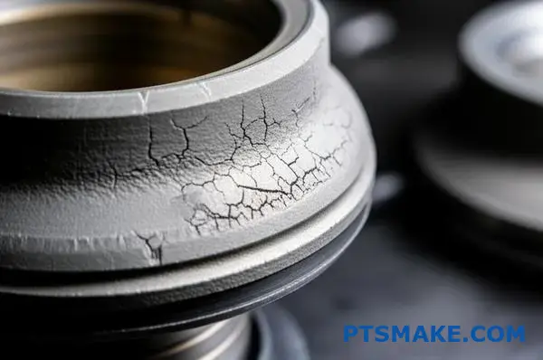
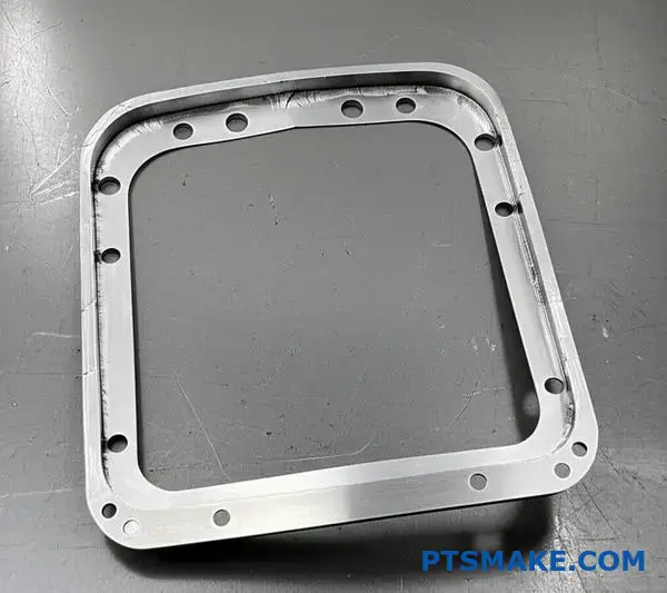
How does surface finish impact fatigue performance?
Fatigue failures almost always start at the surface. It’s the area that interacts with the environment and bears the highest stress.
The Surface: A Critical Starting Point
Tiny surface imperfections act as stress risers. These microscopic cracks grow under repeated loading. This is the core of metal fatigue.
Manufacturing processes directly create this surface. Each method leaves a unique signature. This signature includes roughness and internal stresses. These factors determine the component’s fatigue life.
Manufacturing’s Impact on Fatigue
The table below shows how different finishes affect performance.
| Finishing Process | Typical Roughness (Ra) | Impact on Fatigue Life |
|---|---|---|
| Rough Machining | > 3.2 µm | Poor |
| Grinding | 0.4 – 1.6 µm | Good |
| Polishing | < 0.4 µm | Excellent |
| Shot Peening | Varies | Excellent (induces compression) |
Deeper Dive: Roughness and Residual Stresses
Every manufacturing process alters the surface. Machining, for example, creates microscopic peaks and valleys. These features are prime locations for fatigue cracks to begin. A smoother surface has fewer initiation sites.
Polishing and grinding reduce this roughness. This significantly improves fatigue resistance. However, these processes can also introduce heat and stress into the material.
The most critical factor is the type of stress left behind. We often focus on residual stresses4 that are locked into the surface layer after manufacturing.
Compressive vs. Tensile Stresses
At PTSMAKE, we manage these stresses carefully for our clients. Tensile residual stresses pull the material apart, making it easier for cracks to form. This is detrimental to fatigue life.
Conversely, compressive residual stresses squeeze the material together. This effectively counteracts applied tensile loads, making it much harder for cracks to initiate and grow. Processes like shot peening are designed specifically to create this beneficial effect.
| Process | Typical Residual Stress | Primary Effect on Surface |
|---|---|---|
| Aggressive Grinding | Tensile | Can cause surface damage |
| Gentle Grinding | Compressive/Neutral | Improved finish and life |
| Polishing | Neutral/Slightly Tensile | Very low roughness |
| Shot Peening | Highly Compressive | Increased fatigue strength |
Therefore, specifying the right surface finish is crucial. It’s not just about looks; it is a key engineering requirement for performance.
Fatigue failures originate at the surface. Manufacturing processes dictate the surface’s roughness and residual stress, which are critical factors in determining a component’s resistance to metal fatigue and its overall service life.
What is the fundamental difference between stress and strain control?
Choosing the right control parameter is crucial. It directly impacts the accuracy of fatigue life prediction. The decision depends entirely on the loading conditions.
So, when should you use strain control?
When Deformation is Key
Strain control is best when a part undergoes significant deformation. This is common in situations with large, repeated loads that push the material beyond its elastic limit.
Think of components near stress concentrations. Or parts in thermal cycling. These scenarios often involve notable changes in shape.
High-Cycle vs. Low-Cycle Fatigue
This brings us to a core concept in metal fatigue. The choice between stress and strain control separates two major fatigue regimes.
| Fatigue Type | Controlling Parameter | Typical Cycles to Failure |
|---|---|---|
| High-Cycle Fatigue (HCF) | Stress | > 100,000 |
| Low-Cycle Fatigue (LCF) | Strain | < 100,000 |
In short, for high-cycle, low-stress situations, stress control works well. For low-cycle, high-deformation scenarios, strain control is the reliable choice.
Understanding High-Cycle Fatigue (HCF)
In HCF, the applied stress is low. It stays within the material’s elastic range. This means the component deforms but returns to its original shape after the load is removed.
Because stress and strain remain proportional, using stress as the control parameter is simpler. It provides accurate life predictions for parts experiencing millions of small vibrations, like an engine valve spring.
The Case for Low-Cycle Fatigue (LCF)
LCF is a different story. Here, the loads are high enough to cause significant plastic deformation5. The material permanently changes shape with each cycle.
In this state, the direct link between stress and strain breaks down. Stress is no longer a reliable indicator of the damage being done. Strain—the actual amount of deformation—becomes the critical factor that governs the part’s life.
In past projects at PTSMAKE, especially for aerospace components, getting this distinction right was non-negotiable. A component experiencing LCF, if analyzed using stress control, could fail much earlier than predicted.
| Scenario | Key Characteristic | Best Control Method |
|---|---|---|
| High-Cycle Fatigue | Elastic Deformation | Stress Control |
| Low-Cycle Fatigue | Plastic Deformation | Strain Control |
Our tests confirm that for parts under intense, repetitive loads, a strain-based approach provides a much safer and more accurate prediction of service life.
Strain control is vital for Low-Cycle Fatigue (LCF), where large deformations occur. Stress control is suitable for High-Cycle Fatigue (HCF), where deformation is elastic. This choice is fundamental for accurate fatigue life prediction and ensuring component reliability.
What are the key material properties governing fatigue?
When we talk about fatigue, tensile strength is just the tip of the iceberg. To truly understand a material’s endurance, we must look at more specific properties. These factors predict how a material behaves under repeated stress.
Deeper Fatigue Properties
Understanding these properties is crucial. It allows us to predict component life with much greater accuracy. This is especially true for parts facing complex loading cycles.
Key Coefficients
The main properties we consider are:
- Fatigue Strength Coefficient (σ’f)
- Fatigue Ductility Coefficient (ε’f)
- Cyclic Strain Hardening Exponent (n’)
Here is a quick summary.
| Property | Symbol | Primary Influence |
|---|---|---|
| Fatigue Strength Coefficient | σ’f | High-Cycle Fatigue |
| Fatigue Ductility Coefficient | ε’f | Low-Cycle Fatigue |
| Cyclic Strain Hardening Exponent | n’ | Stress-Strain Response |
These values give us a detailed picture of potential metal fatigue.
These specialized properties are the foundation of modern fatigue analysis. At PTSMAKE, we use them to ensure the parts we manufacture meet strict service life requirements. They are essential inputs for predictive models.
Fatigue Strength Coefficient (σ’f)
This value represents the stress a material can withstand for one load reversal. It primarily governs high-cycle fatigue performance. A higher σ’f generally means better performance in long-life applications. This is where stress levels are low.
Fatigue Ductility Coefficient (ε’f)
This coefficient is the true strain a material can endure for one load reversal. It is critical for low-cycle fatigue. Here, plastic deformation is the main driver of failure. Materials with high ductility often perform better under these conditions.
Cyclic Strain Hardening Exponent (n’)
The n’ value describes how a material’s stress-strain behavior changes under cyclic load. It tells us if the material will get stronger (harden) or weaker (soften) with each cycle. This is vital for using the strain-life approach6 to predict component life.
These properties are not just academic. They directly influence material selection for our clients’ most demanding applications.
| Coefficient | High-Cycle Impact | Low-Cycle Impact |
|---|---|---|
| σ’f (Strength) | Dominant | Minor |
| ε’f (Ductility) | Minor | Dominant |
| n’ (Hardening) | Affects stress response | Affects strain response |
Beyond simple tensile strength, properties like the fatigue strength coefficient, ductility coefficient, and cyclic strain hardening exponent are vital. They provide the necessary data for accurate fatigue life predictions, ensuring component reliability and safety in real-world applications.
When should you use Stress-Life vs. Strain-Life analysis?
Choosing the right fatigue analysis method is crucial. It directly impacts your product’s reliability. The decision boils down to one key factor. You need to know the expected number of cycles and the stress state.
High-Cycle vs. Low-Cycle Fatigue
Stress-Life (S-N) is your go-to for High-Cycle Fatigue (HCF). This applies when a part endures many cycles, over 100,000. Here, stress remains primarily elastic.
Strain-Life (E-N), however, is for Low-Cycle Fatigue (LCF). This is for parts under fewer, but more intense, stress cycles.
A quick comparison helps clarify this:
| Feature | Stress-Life (S-N) | Strain-Life (E-N) |
|---|---|---|
| Fatigue Type | High-Cycle (HCF) | Low-Cycle (LCF) |
| Cycles to Failure | > 10^5 cycles | < 10^5 cycles |
| Material Behavior | Primarily Elastic | Elastic-Plastic |
This distinction is fundamental to avoiding premature failure due to metal fatigue.
Structuring Your Decision
Making the right choice requires looking beyond just cycle count. You must consider the nature of the load and the component’s geometry. This is a common discussion we have with clients at PTSMAKE. We help them select the most appropriate analysis for their parts.
When to Use Stress-Life (S-N)
The S-N method is ideal for components under constant amplitude loading. Think of rotating shafts or vibrating brackets. The stress levels are low enough that the material doesn’t permanently deform. This method is computationally simpler and very effective for long-life applications. It relies on the material’s S-N curve. This curve plots stress amplitude against the number of cycles to failure.
When to Use Strain-Life (E-N)
The E-N method is essential when plastic deformation7 occurs. This happens in areas with high stress concentrations. Examples include notches, holes, or fillets. It is also common in parts experiencing thermal cycling. The analysis focuses on local strain, which is a better predictor of crack initiation in these LCF scenarios.
Here are some typical applications:
| Analysis Method | Typical Applications |
|---|---|
| Stress-Life (S-N) | Engine crankshafts, connecting rods, vehicle suspension components, rotating machinery. |
| Strain-Life (E-N) | Exhaust manifolds, pressure vessels, notched components, turbine blades. |
Choosing the wrong method can lead to inaccurate life predictions. For complex parts, this can be a costly mistake.
Choosing correctly is simple. Use the Stress-Life method for high-cycle applications where stress is elastic. Use the Strain-Life method for low-cycle situations that involve significant plastic strain. This ensures an accurate prediction of component life.
When is a Fracture Mechanics approach necessary?
Linear Elastic Fracture Mechanics (LEFM) operates on a crucial assumption. It assumes a crack already exists in a component.
This changes the engineering question entirely. We no longer ask if a part will fail. We ask how long we have until it does.
The Focus of LEFM
LEFM provides the tools to predict a crack’s behavior. It helps us manage components with known flaws, which is vital in many high-performance applications.
| Approach | Primary Goal | Core Assumption |
|---|---|---|
| Traditional Strength | Prevent crack initiation | The material is perfect |
| LEFM | Manage crack growth | Small flaws already exist |
This approach is the foundation of a damage-tolerant design philosophy. It’s about living with imperfections safely.
The Damage-Tolerant Philosophy
A damage-tolerant philosophy accepts that manufacturing processes or service conditions can introduce small flaws. Instead of aiming for a flawless part, the goal is to ensure these flaws do not grow to a critical size during the component’s service life.
This is a practical and often safer approach. It’s particularly important for industries where failure is not an option, like aerospace and medical devices. This mindset requires a shift from pure strength calculation to life prediction.
Key Metrics in LEFM
Two main concepts drive LEFM: crack propagation rate and remaining useful life.
- Crack Propagation Rate (da/dN): This measures how fast a crack grows with each loading cycle. Understanding this rate is essential when dealing with issues like
metal fatigue. - Remaining Useful Life (RUL): This is the ultimate output. It’s the calculated number of cycles or time a component can operate safely before the existing crack reaches a critical length.
This is the essence of a damage-tolerant design8 philosophy. At PTSMAKE, applying these principles during design reviews helps our clients build more robust and reliable products.
| Step in RUL Analysis | Description | Key Outcome |
|---|---|---|
| 1. Characterize Flaw | Identify or assume an initial crack size. | A defined starting point. |
| 2. Calculate Growth | Use LEFM to model crack propagation. | A prediction of future crack size. |
| 3. Determine End-of-Life | Compare predicted size to critical size. | A clear RUL estimation. |
LEFM provides a robust framework for managing components with existing flaws. By focusing on crack growth rates (da/dN), it allows us to predict the remaining useful life (RUL) and ensure operational safety through a damage-tolerant design philosophy.
What are the major types of environmental fatigue?
Environmental fatigue rarely has a single cause. It’s often a destructive partnership between mechanical stress and a hostile environment.
This teamwork creates what we call synergistic failures. The combined effect is far worse than either factor acting alone.
Key Synergistic Failure Modes
Two primary types dominate this category. These are corrosion fatigue and thermal fatigue. They are critical for engineers to understand.
| Failure Mode | Primary Environmental Factor | Primary Mechanical Factor |
|---|---|---|
| Corrosion Fatigue | Aggressive/Corrosive Media | Cyclic Loading |
| Thermal Fatigue | Cyclic Temperature Changes | Induced Thermal Stress |
Understanding these is key to preventing unexpected metal fatigue failures.
Corrosion Fatigue: A Corrosive Partnership
Corrosion fatigue happens when a part is under cyclic stress in a corrosive environment. Think of a ship’s propeller shaft in saltwater. The saltwater accelerates crack initiation and growth.
The corrosive agent attacks the material surface. It creates pits that act as stress concentrators. This makes it much easier for fatigue cracks to form. The continuous electrochemical reactions9 at the crack tip prevent it from re-welding under compressive loads, speeding up failure.
In past projects at PTSMAKE, we have specified marine-grade stainless steels or specialized coatings to protect components intended for such harsh environments.
Thermal Fatigue: The Hot and Cold Cycle
Thermal fatigue is caused by fluctuating temperatures. When a material is heated, it expands. When cooled, it contracts. If these movements are constrained, internal stresses develop.
Repeated cycles of heating and cooling cause these thermal stresses to eventually initiate cracks. This is a common issue in engine components, like exhaust manifolds or turbine blades. They experience rapid temperature swings during operation.
A key factor is the material’s coefficient of thermal expansion and its thermal conductivity.
| Failure Mode | Common Example | Key Contributing Factors |
|---|---|---|
| Corrosion Fatigue | Offshore Oil Rig Components | Saltwater, acidic rain, industrial chemicals |
| Thermal Fatigue | Automotive Engine Exhaust | High temperature gradients, rapid heating/cooling |
Synergistic failures, like corrosion and thermal fatigue, show how environment and stress combine to weaken materials. Recognizing this interaction is vital for designing durable parts for any application where conditions are not perfect.
How are different metallic alloys classified for fatigue?
Understanding how alloys behave under stress is key. We classify them based on their fatigue response. This is a crucial first step in material selection.
The main division is between ferrous and non-ferrous alloys. This simple classification tells us a lot about potential metal fatigue performance. It guides our initial design choices.
Ferrous vs. Non-Ferrous Behavior
Ferrous alloys, like steel, often have a clear fatigue limit. Non-ferrous alloys, such as aluminum, typically do not.
This distinction is fundamental for predicting part lifetime. Below is a simple breakdown.
| Alloy Type | Fatigue Limit | Implication |
|---|---|---|
| Ferrous (e.g., Steel) | Often has a distinct limit | Can endure infinite cycles below this limit |
| Non-Ferrous (e.g., Aluminum) | Typically no distinct limit | Will eventually fail, regardless of stress level |
This difference dictates how we design for long-term durability.

This classification has major implications for design. It’s not just theory; it directly impacts safety, cost, and performance. In past projects at PTSMAKE, choosing the right category saved clients from costly redesigns.
The Role of the S-N Curve
The Stress-Life, or S-N Curve10, graphically shows this behavior. For steel, the curve often becomes horizontal. This flat portion represents the endurance limit. If stress cycles stay below this level, the part theoretically lasts forever.
Non-ferrous alloys like aluminum and titanium show a continuously sloping S-N curve. This means that any stress cycle, no matter how small, contributes to eventual failure. This requires a different design philosophy, often called "safe-life" or "damage-tolerant" design.
Industry-Specific Applications
Different industries prioritize different factors. This directly influences their alloy classification choices. The automotive industry often uses steel for its cost-effectiveness and high endurance limit.
Aerospace, however, prioritizes a high strength-to-weight ratio. They frequently use aluminum and titanium alloys. Engineers must carefully calculate the component’s finite lifespan.
Here’s how this plays out in practice.
| Industry | Primary Material Focus | Design Philosophy | Key Consideration |
|---|---|---|---|
| Automotive | Ferrous Alloys (Steel) | Infinite Life (Endurance Limit) | Cost and High-Volume Production |
| Aerospace | Non-Ferrous Alloys (Al, Ti) | Safe-Life / Damage-Tolerant | Weight Reduction and Safety |
This shows why a one-size-fits-all approach to metal fatigue doesn’t work.
Classifying alloys by fatigue behavior—specifically ferrous versus non-ferrous—is critical. This distinction shapes design philosophy, material selection, and lifecycle predictions, with major implications for industries like automotive and aerospace, guiding engineers to make safe and effective choices.
What constitutes high-cycle versus low-cycle fatigue (LCF)?
The line between High-Cycle Fatigue (HCF) and Low-Cycle Fatigue (LCF) is blurry if you only look at cycle counts. The real difference is how the material behaves under load. It’s about the dominant deformation mechanism.
The Core Distinction
HCF is driven by stress. The material flexes but remains within its elastic limits. Think of a spring bouncing back every time.
In contrast, LCF is driven by strain. The material experiences plastic deformation, meaning it permanently changes shape with each cycle. This is a key factor in metal fatigue.
HCF vs. LCF at a Glance
| Feature | High-Cycle Fatigue (HCF) | Low-Cycle Fatigue (LCF) |
|---|---|---|
| Driver | Stress | Strain |
| Deformation | Elastic | Plastic |
| Load Level | Low | High |
Stress-Driven vs. Strain-Driven Failure
Thinking in terms of deformation gives you a much clearer picture. It helps us predict failure more accurately. This is a concept we apply daily at PTSMAKE when designing parts for long-term reliability.
High-Cycle Fatigue (HCF): Living in the Elastic Zone
In HCF, the applied stress is below the material’s yield strength. The component experiences millions, or even billions, of cycles before failure.
Because deformation is elastic, the part returns to its original shape after each load cycle. The damage accumulates very slowly. This is typical for parts experiencing vibration.
Low-Cycle Fatigue (LCF): The Impact of Plasticity
LCF occurs when stress levels exceed the material’s yield strength. This causes plasticity11, or permanent deformation, in each cycle. The part doesn’t fully spring back.
This plastic strain is the primary cause of damage. It accumulates much faster, leading to failure in a lower number of cycles, often less than 100,000.
In our past projects, we’ve found that LCF is best described by strain-based models. A key one is the Coffin-Manson relationship. It links plastic strain to the number of cycles to failure. This model is crucial for designing components like pressure vessels or aircraft landing gear.
The key is understanding the mechanism. HCF is a stress-driven, elastic phenomenon. LCF is a strain-driven process dominated by plastic deformation. This distinction is far more important for predicting part lifespan than a simple cycle count.
What are the main categories of fatigue life enhancement techniques?
To tackle component failure, we can group enhancement techniques into three main areas. This approach helps us systematically improve product durability. It’s about being smart from the start.
Each category addresses failure from a different angle. This provides a comprehensive strategy against metal fatigue.
Geometric Design
We start by shaping the part to reduce stress. Sharp corners are weak points. Smooth transitions and larger radii distribute loads more evenly.
Material Selection
Choosing the right material is fundamental. Factors like strength, ductility, and resistance to crack growth are critical for performance.
Surface Treatments
These methods modify the component’s surface. They create a protective layer that resists crack initiation, boosting fatigue life significantly.
| Category | Primary Goal | Common Application |
|---|---|---|
| Geometric Design | Reduce Stress Concentration | Filleting sharp corners |
| Material Selection | Increase Intrinsic Resistance | Using high-strength alloys |
| Surface Treatments | Induce Compressive Stress | Shot peening surfaces |

Improving fatigue life requires a multi-faceted approach. At PTSMAKE, we don’t just focus on one method. We combine them for the best results. A well-designed part made from a superior material and then properly treated will always outperform one that only gets one aspect right.
Smart Geometric Design
The goal is to eliminate stress concentration factors. This means designing smooth transitions, generous fillets, and polished surfaces. Every sharp notch or hole acts as a starting point for a crack. We always review designs to smooth out these high-risk areas before machining begins.
Choosing the Right Material
Material choice goes beyond just strength. We consider toughness and how the material behaves under cyclic loading. Some materials are better at resisting crack growth than others. The material’s internal structure and potential for anisotropy12 also play a huge role in its overall fatigue performance. Our material experts help clients select the optimal grade for their specific application.
Applying Surface Treatments
Surface treatments are a powerful tool. They introduce compressive residual stresses on the surface. This stress must be overcome before a crack can even start to form. Based on our tests, techniques like shot peening or case hardening can dramatically extend the life of a component.
| Technique Category | Specific Method | How It Works |
|---|---|---|
| Geometric Design | Filleting & Radiusing | Smoothens stress flow |
| Stress Relief Grooves | Redirects stress from critical areas | |
| Material Selection | High-Purity Alloys | Reduces inclusions that initiate cracks |
| Forged Materials | Aligns grain structure for strength | |
| Surface Treatment | Shot Peening | Creates surface compressive stress |
| Case Hardening | Hardens the surface layer |
In summary, enhancing fatigue life isn’t about a single magic fix. It’s a strategic combination of thoughtful geometric design, appropriate material selection, and targeted surface treatments. This holistic approach ensures maximum component reliability and longevity.
How do welded joints alter fatigue analysis?
Welded joints are often the weakest link in fatigue analysis. They introduce a complex mix of issues that significantly reduce a component’s life.
The Triple Threat in Welds
Welds create geometric discontinuities. These act as stress raisers. The welding process also changes the material’s properties locally.
This combination makes welds prime locations for crack initiation. Understanding these factors is crucial for accurate fatigue life prediction.
Key Factors Altering Fatigue Life
| Factor | Description | Impact on Fatigue |
|---|---|---|
| Geometric Notches | Sharp changes at the weld toe and root. | High-stress concentration. |
| Metallurgical Changes | Heat-Affected Zone (HAZ) formation. | Altered, often brittle, material. |
| Residual Stresses | Stresses locked in after cooling. | Acts as a constant tensile load. |
These elements work together, accelerating metal fatigue.

Welds introduce a perfect storm for fatigue failure. It’s not just one issue, but three acting together. This complexity is why standard fatigue analysis often falls short for welded structures.
Geometric Stress Concentrators
The weld toe and root are natural stress concentrators. The abrupt change in shape at these points magnifies the applied stress. Even a perfectly executed weld has these features. They act as built-in starting points for fatigue cracks.
Metallurgical Transformations
The intense heat from welding creates a Heat-Affected Zone (HAZ). In this zone, the base metal’s microstructure13 is altered without being melted. Based on project experience, this often results in a harder, more brittle material. This brittleness makes the HAZ highly susceptible to cracking under cyclic loads.
| Zone | Hardness | Ductility | Fatigue Resistance |
|---|---|---|---|
| Base Metal | Normal | High | High |
| HAZ | Increased | Reduced | Low |
| Weld Metal | Varies | Varies | Varies |
The Impact of Residual Stresses
As the weld cools, it contracts. This contraction is restrained by the surrounding cooler metal. This process locks in high tensile residual stresses. These stresses can be as high as the material’s yield strength. They act like a constant mean stress, significantly accelerating fatigue crack growth.
Welded joints introduce a trifecta of fatigue risks: geometric notches, brittle material zones, and high tensile residual stresses. This combination makes them critical hotspots that demand special attention in any durable design, a lesson we apply daily at PTSMAKE.
What are the common fatigue analysis software workflows?
Computer-Aided Engineering (CAE) provides a structured workflow for fatigue analysis. This process is essential for predicting a component’s lifespan under operational loads. It helps us prevent failures before they happen.
The entire process is data-driven. It starts with a digital model and ends with a life prediction.
The Typical CAE Structure
Step 1: Finite Element Analysis (FEA)
First, we use FEA software. This helps identify stress hotspots on the part. These are the areas most likely to fail.
Step 2: Key Inputs
Next, we define the core data for the simulation. This involves material properties and loading conditions. The accuracy of this data is critical for reliable results.
| Input Type | Description |
|---|---|
| Material Properties | S-N curve data defining fatigue resistance. |
| Loading Histories | Real-world force, pressure, or vibration data. |
Step 3: Fatigue Solver
Finally, a dedicated solver calculates the results. It combines all the data to predict component life and damage accumulation.
The CAE workflow is powerful, but its output is only as good as its input. In past projects at PTSMAKE, we’ve seen that small errors in initial data can lead to significant miscalculations in predicted life.
Diving Deeper into the Workflow
The Importance of Accurate Inputs
The most critical phase is data collection. FEA results show where stress is highest. But material and load data tell the solver how the part will respond to that stress over time. This is fundamental to understanding potential metal fatigue.
Defining Material Behavior
We define a material’s fatigue properties using specific data curves. These curves are often generated from extensive physical testing. They detail how a material behaves under cyclic stress.
Translating Real-World Loads
Loading histories are rarely simple sine waves. They are often complex and variable. We use algorithms like Rainflow counting14 to process this messy, real-world data into a format the solver can understand. This step is crucial for accurate life prediction.
The Solver’s Calculation
The fatigue solver acts as the final calculator. It takes the stress results from FEA, applies the loading history, and references the material’s fatigue properties to predict total life.
| Stage | Primary Function | Output |
|---|---|---|
| FEA | Identifies stress concentrations. | Stress/Strain Maps |
| Fatigue Solver | Calculates damage accumulation. | Predicted Life (Cycles/Hours) |
The standard CAE fatigue workflow is a multi-stage process. It integrates FEA for stress analysis, precise material and load data for context, and a specialized solver to calculate the final fatigue life, ensuring a comprehensive durability assessment.
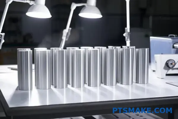
How do you design a standard fatigue test program?
Creating a reliable S-N curve is essential for predicting a material’s life. It’s a foundational step in any fatigue analysis. The process must be systematic.
It starts with carefully designed specimens. These must represent the final part accurately.
Initial Planning Stage
Next, we select appropriate stress levels. This range determines the scope of our curve. A poor selection can lead to useless data.
Here are the first key steps:
| Step | Description |
|---|---|
| Specimen Design | Create samples that mimic the final product’s geometry. |
| Stress Level Selection | Choose multiple stress levels to test life cycles. |
This initial phase sets the foundation for accurate results.
Test Execution and Data Fitting
After setting the stage, we determine how many specimens to test at each stress level. More specimens provide greater statistical confidence. This helps us understand the material’s variability.
We also need to define the runout criteria15. This is the cycle count at which we consider a specimen to have infinite life. It stops tests from running forever.
At PTSMAKE, we understand specimen consistency is key. Our precision CNC machining ensures test results are reliable. They are not skewed by manufacturing defects. Poor specimens can completely invalidate expensive testing programs.
Once testing is complete, we analyze the data. This involves statistically fitting the stress and life data points. This creates the final design curve. It is a vital tool for predicting metal fatigue.
| Analysis Phase | Key Action |
|---|---|
| Specimen Count | Test multiple samples per stress level for accuracy. |
| Runout Definition | Set a cycle limit for "infinite" life. |
| Statistical Fitting | Use methods like linear regression to create the curve. |
This systematic approach transforms raw data into actionable engineering insights for preventing component failure.
Generating a reliable S-N curve is a multi-step process. It starts with precise specimen design and stress level selection, followed by rigorous testing and statistical data fitting. This creates the final design curve for fatigue life prediction.
How do you implement a fatigue design improvement strategy?
When a component fails prematurely, guessing isn’t a strategy. A structured framework is the only reliable way forward. This approach turns a critical failure into a valuable learning opportunity.
A Framework for Problem-Solving
We must systematically diagnose the problem. This ensures we find the true root cause. It prevents costly repeat failures. This structured process is key to improving product reliability and managing metal fatigue.
A clear, step-by-step method is essential.
| Step | Focus Area |
|---|---|
| 1 | Confirm Failure Mode |
| 2 | Understand Operating Loads |
| 3 | Analyze and Replicate |
| 4 | Develop Solutions |
| 5 | Validate the Improvement |
This methodical approach builds confidence in the final solution.
Diving Into the Process
Let’s explore each step more closely. At PTSMAKE, we’ve refined this process over many projects. A disciplined approach always delivers the best results. It avoids costly detours and assumptions.
Step 1: Failure Analysis
The first task is to confirm fatigue as the failure mechanism. This involves a detailed examination of the fractured component. The process of Fractography16 allows us to read the story of how the crack initiated and grew over time.
Step 2: Load Data Acquisition
Next, we need to understand the real-world conditions. We often attach sensors or strain gauges to components in service. This provides precise data on the loads, frequencies, and environmental factors the part actually endures.
Step 3 & 4: Analysis and Solutions
With accurate load data, we use analysis software to build a model that replicates the failure. Once our model matches reality, we can test potential solutions digitally.
| Improvement Strategy | Primary Benefit | Consideration |
|---|---|---|
| Geometry Change | Reduces stress concentration | May impact assembly |
| Material Change | Increases intrinsic strength | Cost and availability |
| Surface Treatment | Induces compressive stress | Adds process step/cost |
Step 5: Validation
Finally, any proposed fix must be rigorously validated. This might involve accelerated life testing in a lab or a carefully monitored field test. Validation is the ultimate proof that the problem is solved.
A structured five-step framework transforms fatigue failure from a crisis into a solvable engineering problem. It guides the process from analysis and data collection to proposing and, most importantly, validating a robust, permanent solution for the component.
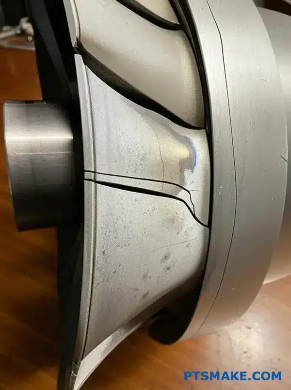
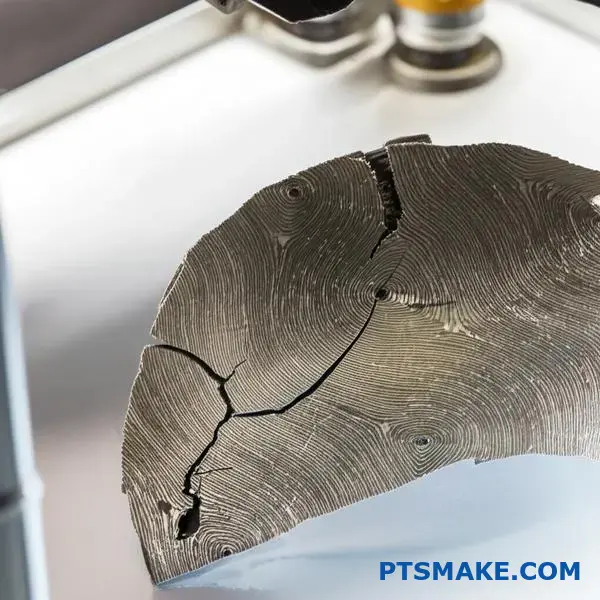
How do you interpret fatigue fractography results?
Reading a fracture surface tells the complete story of a part’s failure. It’s a critical step in any failure analysis. The surface reveals where the problem started and how it progressed.
By identifying key features, we can pinpoint the root cause of the metal fatigue. This helps prevent future failures.
Key Features on a Fracture Surface
A typical fatigue fracture has three distinct zones. Each zone provides clues about the failure timeline.
| Feature | Location | What It Tells Us |
|---|---|---|
| Initiation Site | Origin of the crack | The root cause (e.g., stress concentration) |
| Propagation Zone | Middle section | History of crack growth under loading |
| Fast Fracture Zone | Final section | The point of catastrophic overload |
Understanding these zones is essential. It allows us to build more reliable parts.
Deeper Analysis of Fracture Features
Interpreting these features goes beyond simple identification. The details provide crucial insights into the failure conditions.
The Initiation Site’s Story
The crack’s origin is the most important clue. If it starts at a sharp corner or a hole, it points to a design issue creating a stress concentration. At PTSMAKE, we always review designs to minimize these risks.
If the origin is a material defect like an inclusion, it points to a material quality problem. This guides our material selection and sourcing processes.
Reading the Propagation Zone
The propagation zone is marked by "beachmarks" or "clamshell marks." These concentric lines show the crack’s progression.
Closely spaced beachmarks indicate slow crack growth. This might happen under low, consistent stress. Widely spaced marks suggest higher stress cycles or a more corrosive environment. On a microscopic level, you might see striations17, where each line corresponds to a single load cycle.
This information helps us understand the real-world loading conditions the part experienced.
| Beachmark Spacing | Likely Cause |
|---|---|
| Close | Slow crack growth, lower stress |
| Wide | Faster growth, higher stress cycles |
The Final Overload
The fast fracture zone is typically rough and crystalline. Its size relative to the rest of the surface is very telling.
A small fast fracture zone means the crack grew slowly over a long time until the remaining material could no longer support the load. A large fast fracture zone indicates the final break happened under a very high load.
Interpreting a fracture surface means identifying the crack origin, propagation patterns like beachmarks, and the final fracture zone. This analysis reveals the failure’s root cause, guiding better design and material choices to prevent recurrence.
Analyze a classic failure: the de Havilland Comet crashes.
The de Havilland Comet was a pioneer. It ushered in the age of commercial jet travel. However, a series of tragic crashes exposed a deep flaw hidden within its groundbreaking design.
This story is a crucial lesson for every engineer and manufacturer. It demonstrates how seemingly small design details can result in catastrophic failure.
Core Issues of the Comet Failure
- Design Element: The use of square windows.
- Operational Stress: High-altitude cabin pressurization cycles.
- Root Cause: A critical misunderstanding of metal fatigue.
Let’s dissect the engineering missteps that led to this disaster.
The Comet’s failure wasn’t due to a single error. It was a chain reaction of design choices and unknown material behaviors. At PTSMAKE, our projects often reinforce the lesson that every detail, no matter how small, contributes to the final product’s integrity.
Stress Concentration at Square Windows
The sharp corners of the Comet’s square windows were the fatal flaw. These corners acted as stress concentrators. Each time the plane reached cruising altitude, the cabin was pressurized, and it was depressurized during descent.
This constant expansion and contraction created what we call cyclic loading18 on the aluminum fuselage skin. The stresses were highest at those sharp corners.
Deconstructing the Failure Process
Investigators eventually pieced together the sequence of events. The repeated stress cycles caused metal fatigue. This led to microscopic cracks forming at rivet holes near the window corners.
With every flight, these cracks grew just a little bit. They were invisible to the naked eye until it was too late. Finally, a crack reached a critical length, causing the fuselage to tear apart in mid-air.
| Failure Component | Role in the Disaster |
|---|---|
| Stress Concentrator | Sharp corners of the windows |
| Load Type | Repeated cabin pressurization cycles |
| Failure Mechanism | Metal fatigue crack initiation and propagation |
| Initiation Site | Rivet holes at the highest stress points |
The Comet disaster was a wake-up call for the entire aviation industry. It led to mandatory, rigorous fatigue testing of aircraft structures and is the reason all aircraft windows are oval today.
The Comet crashes taught a painful but vital lesson. Stress concentration from square windows, combined with the effects of cyclic pressurization and an underestimation of metal fatigue, created a perfect storm for failure. This tragedy fundamentally reshaped aviation design and safety standards.
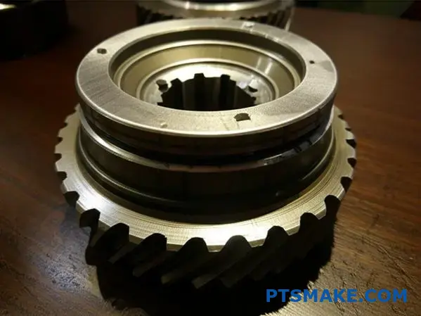
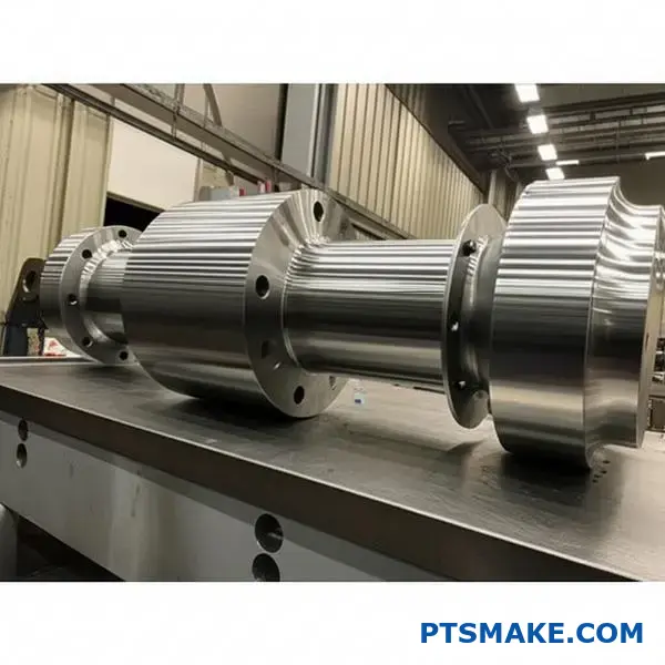
Design a fatigue-resistant axle for a freight railcar.
Designing a freight railcar axle is a great simulation of a real-world project. It’s not just about strength; it’s about endurance. The axle must resist failure over millions of cycles.
Our process starts with defining the loads. We then select the right material. Finally, we optimize the geometry and calculate its fatigue life. This ensures the axle meets service life requirements without failing.
Key Design Stages
| Stage | Objective | Method |
|---|---|---|
| 1. Load Definition | Capture real-world variable stresses | Loading Spectrum Analysis |
| 2. Material Selection | Ensure strength and toughness | Material Property Evaluation |
| 3. Geometry Optimization | Minimize stress concentrations | Finite Element Analysis (FEA) |
| 4. Life Calculation | Verify service life | Fatigue Life Analysis |
A Closer Look at the Design Process
Let’s break down the design simulation further. Defining the loading spectrum is the most critical first step. We must account for variable loads from track imperfections, curves, and braking forces. These unpredictable loads are the primary cause of metal fatigue.
Material and Geometry
For a demanding application like this, forged steel is a superior choice. Its grain structure provides excellent toughness and resistance to crack propagation. At PTSMAKE, we often machine high-strength forged materials for clients in demanding industries.
Next, we use Finite Element Analysis (FEA). We focus on high-stress areas like the bearing journals. FEA helps us optimize the fillet radii and diameter transitions. This reduces stress concentrations, which are the starting points for fatigue cracks. Our analysis has shown that even small geometric adjustments can significantly increase axle life.
Ensuring Longevity
Finally, a simple stress check is not enough. We perform a detailed fatigue life calculation. This involves summing the damage from all the different load cycles. To do this, we use a method like Miner’s rule19 to ensure the axle’s cumulative damage is below the failure threshold for its entire service life.
| Design Factor | Importance | Optimization Tool |
|---|---|---|
| Variable Loads | High | Spectrum Analysis |
| Material Choice | High | Material Science |
| Stress Hotspots | High | FEA Software |
| Cumulative Damage | High | Life Calculation Formulas |
This process—defining loads, selecting materials, optimizing geometry with FEA, and calculating fatigue life—is essential. It ensures a freight railcar axle is both strong and incredibly durable, preventing catastrophic failures and ensuring operational safety for the long haul.
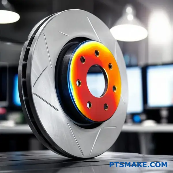
How does temperature affect your entire fatigue analysis workflow?
Integrating thermal effects is a non-negotiable step. It is not a simple add-on. Temperature fundamentally alters your entire fatigue analysis.
Elevated temperatures directly impact how a material behaves. Ignoring this can lead to catastrophic, unexpected failures.
Reduced Material Strength
As temperatures increase, most metals soften. Their ability to withstand cyclic loads decreases. This can significantly shorten a component’s service life. We must account for this degradation.
Complex Damage Mechanisms
New failure modes like creep and thermal cycling also appear. These introduce complex, strain-driven damage that standard analysis often misses.
| Temperature Effect | Impact on Fatigue Analysis |
|---|---|
| Lower Yield Strength | Requires updated S-N curves |
| Increased Ductility | Affects strain-life models |
| Creep Deformation | Introduces time-dependency |
So, how do you properly adapt your workflow? The entire process begins with gathering the right data. Your standard room-temperature material properties are no longer sufficient for accurate predictions.
Temperature-Dependent Material Data
You need material data across the full operating temperature range. This includes temperature-specific S-N curves, E-N curves, and creep data. Without this, your analysis is just a guess.
At PTSMAKE, we often collaborate with clients to test materials under operational conditions. This ensures our analysis is grounded in real-world performance, not just textbook values.
Modifying the Analysis Process
Your analysis must account for these combined effects. This involves considering both mechanical and thermal loads simultaneously, not in isolation. A sequential or fully coupled analysis is often necessary.
Thermal cycling introduces strain that must be added to the mechanical strain. This complex interaction is often modeled using specific damage accumulation rules, which sometimes incorporate principles like the Arrhenius equation20 for rate-dependent processes like creep.
| Analysis Step | Standard Approach | Modified for Temperature |
|---|---|---|
| Material Data | Room Temp S-N Curve | Temp-dependent properties |
| Loading | Mechanical cycles only | Mechanical + Thermal cycles |
| Damage Model | Miner’s Rule | Creep-fatigue interaction models |
Temperature fundamentally alters fatigue analysis. It reduces material strength and introduces complex failure modes. Adapting your workflow requires using temperature-dependent material data and advanced models that account for both mechanical and thermal loads to ensure accurate life predictions.
Unlock Metal Fatigue Solutions with PTSMAKE Expertise
Ready to ensure unmatched fatigue resistance and durability for your next project? Contact PTSMAKE now for a tailored quote on precision CNC machining or injection molding. Let our expertise in metal fatigue and quality manufacturing give you the confidence you need—from prototype to production.

Explore a detailed explanation of how these microscopic bands form and lead to component failure. ↩
Learn how this key material property influences fatigue life predictions in S-N analysis. ↩
Learn how different materials respond to stress risers, a key factor in component design and material selection. ↩
Explore how internal stresses impact material strength, even without external loads. ↩
Understand how materials permanently change shape under load and why it’s critical for fatigue analysis. ↩
Explore this key model for predicting fatigue life under complex loading conditions. ↩
Learn how permanent changes in a material’s shape impact fatigue life and part performance. ↩
Learn how this design approach prioritizes safety by assuming flaws exist. ↩
Learn more about the chemical processes that accelerate corrosion fatigue and how to mitigate them. ↩
Click to learn more about the S-N Curve and its importance in fatigue analysis and material selection. ↩
Understand how permanent deformation under load impacts material lifespan and part design. ↩
Understand how a material’s properties can vary with direction and affect fatigue strength. ↩
See how material microstructure directly influences component strength and overall fatigue life. ↩
Learn how this algorithm simplifies complex load histories into countable stress cycles for analysis. ↩
Discover how setting this test parameter is crucial for infinite life assessment. ↩
Learn how examining fracture surfaces helps identify the root cause of material failure. ↩
Discover the difference between macroscopic beachmarks and the microscopic lines that mark single stress cycles. ↩
Understand how repeated stress, even below a material’s ultimate strength, can lead to failure. ↩
Learn how this rule estimates cumulative fatigue damage under variable loading conditions. ↩
Understand the core equation for modeling how temperature accelerates material degradation and creep phenomena. ↩